Going Rogue: The Search for Anything (and Everything) with ATLAS

Title: “A model-independent general search for new phenomena with the ATLAS detector at √s=13 TeV”

Author: The ATLAS Collaboration

Reference: ATLAS-PHYS-CONF-2017-001


When a single experimental collaboration has a few thousand contributors (and even more opinions), there are a lot of rules. These rules dictate everything from how you get authorship rights to how you get chosen to give a conference talk. In fact, this rulebook is so thorough that it could be the topic of a whole other post. But for now, I want to focus on one rule in particular, a rule that has only been around for a few decades in particle physics but is considered one of the most important practices of good science: blinding.

In brief, blinding is the notion that it’s experimentally compromising for a scientist to look at the data before finalizing the analysis. As much as we like to think of ourselves as perfectly objective observers, the truth is, when we really really want a particular result (let’s say a SUSY discovery), that desire can bias our work. For instance, imagine you were looking at actual collision data while you were designing a signal region. You might unconsciously craft your selection in such a way to force an excess of data over background prediction. To avoid such human influences, particle physics experiments “blind” their analyses while they are under construction, and only look at the data once everything else is in place and validated.

Figure 1: “Blind analysis: Hide results to seek the truth”, R. MacCounor & S. Perlmutter for Nature.com

This technique has kept the field of particle physics in rigorous shape for quite a while. But there’s always been a subtle downside to this practice. If we only ever look at the data after we finalize an analysis, we are trapped within the confines of theoretically motivated signatures. In this blinding paradigm, we’ll look at all the places that theory has shone a spotlight on, but we won’t look everywhere. Our whole game is to search for new physics. But what if amongst all our signal regions and hypothesis testing and neural net classifications… we’ve simply missed something?

It is this nagging question that motivates a specific method of combing the LHC datasets for new physics, one that the authors of this paper call a “structured, global and automated way to search for new physics.” With this proposal, we can let the data itself tell us where to look and throw unblinding caution to the winds.

The idea is simple: scan the whole ATLAS dataset for discrepancies, setting a threshold for what defines a feature as “interesting”. If this preliminary scan stumbles upon a mysterious excess of data over Standard Model background, don’t just run straight to Stockholm proclaiming a discovery. Instead, simply remember to look at this area again once more data is collected. If your feature of interest is a fluctuation, it will wash out and go away. If not, you can keep watching it until you collect enough statistics to do the running to Stockholm bit. Essentially, you let a first scan of the data rather than theory define your signal regions of interest. In fact, all the cool kids are doing it: H1, CDF, D0, and even ATLAS and CMS have performed earlier versions of this general search.

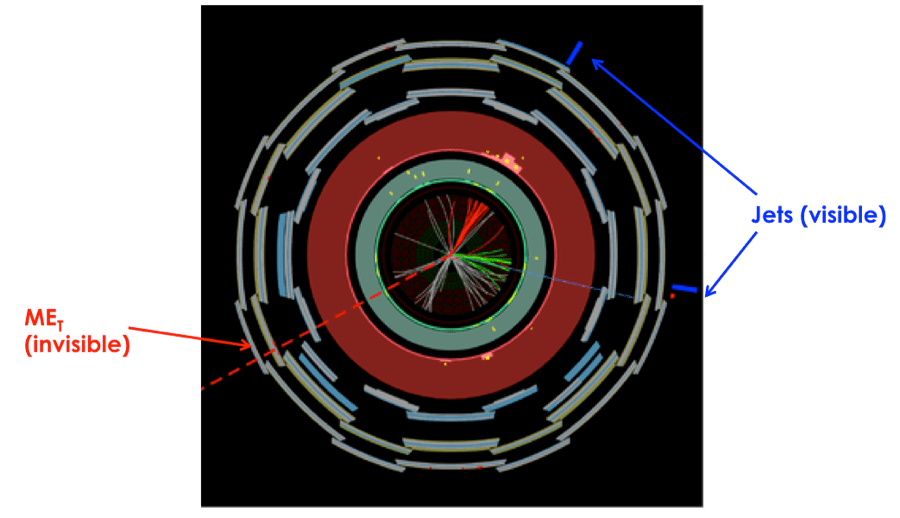
The nuts and bolts of this particular paper include 3.2 fb-1 of 2015 13 TeV LHC data to try out. Since the whole goal of this strategy is to be as general as possible, we might as well go big or go home with potential topologies. To that end, the authors comb through all the data and select any event “involving high pT isolated leptons (electrons and muons), photons, jets, b-tagged jets and missing transverse momentum”. All of the backgrounds are simply modeled with Monte Carlo simulation.

Once we have all these events, we need to sort them. Here, “the classification includes all possible final state configurations and object multiplicities, e.g. if a data event with seven reconstructed muons is found it is classified in a ‘7- muon’ event class (7μ).” When you add up all the possible permutations of objects and multiplicities, you come up with a cool 639 event classes with at least 1 data event and a Standard Model expectation of at least 0.1.

From here, it’s just a matter of checking data vs. MC agreement and the pulls for each event class. The authors also apply some measures to weed out the low stat or otherwise sketchy regions; for instance, 1 electron + many jets is more likely to be multijet faking a lepton and shouldn’t necessarily be considered as a good event category. Once this logic applied, you can plot all of your SRs together grouped by category; Figure 2 shows an example for the multijet events. The paper includes 10 of these plots in total, with regions ranging in complexity from nothing but 1μ1j to more complicated final states like ETmiss2μ1γ4j (say that five times fast.)

Figure 2: The number of events in data and for the different SM background predictions considered. The classes are labeled according to the multiplicity and type (e, μ, γ, j, b, ETmiss) of the reconstructed objects for this event class. The hatched bands indicate the total uncertainty of the SM prediction.


Once we can see data next to Standard Model prediction for all these categories, it’s necessary to have a way to measure just how unusual an excess may be. The authors of this paper implement an algorithm that searches for the region of largest deviation in the distributions of two variables that are good at discriminating background from new physics. These are the effective massthe sum of all jet and missing momenta, and the invariant mass, computed with all visible objects and no missing energy.

For each deviation found, a simple likelihood function is built as the convolution of probability density functions (pdfs): one Poissonian pdf to describe the event yields, and Gaussian pdfs for each systematic uncertainty. The integral of this function, p0, is the probability that the Standard Model expectation fluctuated to the observed yield. This p0 value is an industry standard in particle physics: a value of p0 < 3e-7 is our threshold for discovery.

Sadly (or reassuringly), the smallest p0 value found in this scan is 3e-04 (in the 1m1e4b2j event class). To figure out precisely how significant this value is, the authors ran a series of pseudoexperiments for each event class and applied the same scanning algorithm to them, to determine how often such a deviation would occur in a wholly different fake dataset. In fact, a p0 of 3e-04 was expected 70% of the pseudoexperiments.

So the excesses that were observed are not (so far) significant enough to focus on. But the beauty of this analysis strategy is that this deviation can be easily followed up with the addition of a newer dataset. Think of these general searches as the sidekick of the superheros that are our flagship SUSY, exotics, and dark matter searches. They can help us dot i’s and cross t’s, make sure nothing falls through the cracks— and eventually, just maybe, make a discovery.

Grad students can apply now for ComSciCon’18!

Applications are now open for the Communicating Science 2018 workshop, to be held in Boston, MA on June 14-16, 2018!

Graduate students at U.S. and Canadian institutions in all fields of science, technology, engineering, health, mathematics, and related fields are encouraged to apply. The application deadline is March 1st.

Graduate student attendees of ComSciCon’17

As for past ComSciCon national workshops, acceptance to the workshop is competitive; attendance is free and travel support and lodging will be provided to accepted applicants.

Attendees will be selected on the basis of their achievement in and capacity for leadership in science communication. Graduate students who have engaged in entrepreneurship and created opportunities for other students to practice science communication are especially encouraged to apply.

Participants will network with other leaders in science communication and build the communication skills that scientists and other technical professionals need to express complex ideas to the general public, experts in other fields, and their peers. In additional to panel discussions on topics like Science Journalism, Creative & Digital Storytelling, and Diversity and Inclusion in Science, ample time is allotted for networking with science communication experts and developing science outreach collaborations with fellow graduate students.

You can follow this link to submit an application or learn more about the workshop programs and participants. You can also follow ComSciCon on Twitter (@comscicon) and use #comscicon18 !

Our group photo at ComSciCon’17

Longtime Astrobites readers may remember that ComSciCon was founded in 2012 by Astrobites and Chembites authors. Since then, we’ve led five national workshops on leadership in science communication and established a franchising model through which graduate student alums of our program have led sixteen regional and specialized workshops on training in science communication.

We are so excited about the impact ComSciCon has had on the science communication community. You can read more about our programs, the outcomes we have documented, find vignettes about our amazing graduate student attendees, and more in ComSciCon’s 2017 annual report.

The organizers of ComSciCon’17. Can you spot the astronomers?

None of ComSciCon’s impacts would be possible without the generous support of our sponsors. These contributions make it possible for us to offer this programming free of charge to graduate students, and to support their travel to our events. In particular, we wish to thank the American Astronomical Society for being a supporter of both Particlebites and ComSciCon.

If you believe in the mission of ComSciCon, you can support our program to! Visit our webpage to learn more and donate today!

Attendees react to a challenging section of a student’s Pop Talk at ComSciCon’17

A Moriond Retrospective: New Results from the LHC Experiments

Hi ParticleBiters!

In lieu of a typical HEP paper summary this month, I’m linking a comprehensive overview of the new results shown at this year’s Moriond conference, originally published in the CERN EP Department Newsletter. Since this includes the latest and greatest from all four experiments on the LHC ring (ATLAS, CMS, ALICE, and LHCb), you can take it as a sort of “state-of-the-field”. Here is a sneak preview:

“Every March, particle physicists around the world take two weeks to promote results, share opinions and do a bit of skiing in between. This is the Moriond tradition and the 52nd iteration of the conference took place this year in La Thuile, Italy. Each of the four main experiments on the LHC ring presented a variety of new and exciting results, providing an overview of the current state of the field, while shaping the discussion for future efforts.”

Read more in my article for the CERN EP Department Newsletter here!

The integrated luminosity of the LHC with proton-proton collisions in 2016 compared to previous years. Luminosity is a measure of a collider’s performance and is proportional to the number of collisions. The integrated luminosity achieved by the LHC in 2016 far surpassed expectations and is double that achieved at a lower energy in 2012.


Why Electroweak SUSY is the Next Big Thing

Title: “Search for new physics in events with two low momentum opposite-sign leptons and missing transverse energy at s = 13 TeV”

Author: CMS Collaboration

Reference: CMS-PAS-SUS-16-048


March is an exciting month for high energy physicists. Every year at this time, scientists from all over the world gather for the annual Moriond Conference, where all of the latest results are shown and discussed. Now that this physics Christmas season is over, I, like many other physicists, am sifting through the proceedings, trying to get a hint of what is the new cool physics to be chasing after. My conclusions? The Higgsino search is high on this list.

Physicists chatting at the 2017 Moriond Conference. Image credit ATLAS-PHOTO-2017-009-1.

The search for Higgsinos falls under the broad and complex umbrella of searches for supersymmetry (SUSY). We’ve talked about SUSY on Particlebites in the past; see a recent post on the stop search for reference. Recall that the basic prediction of SUSY is that every boson in the Standard Model has a fermionic supersymmetric partner, and every fermion gets a bosonic partner.

So then what exactly is a Higgsino? The naming convention of SUSY would indicate that the –ino suffix means that a Higgsino is the supersymmetric partner of the Higgs boson. This is partly true, but the whole story is a bit more complicated, and requires some understanding of the Higgs mechanism.

To summarize, in our Standard Model, the photon carries the electromagnetic force, and the W and Z carry the weak force. But before electroweak symmetry breaking, these bosons did not have such distinct tasks. Rather, there were three massless bosons, the B, W, and Higgs, which together all carried the electroweak force. It is the supersymmetric partners of these three bosons that mix to form new mass eigenstates, which we call simply charginos or neutralinos, depending on their charge. When we search for new particles, we are searching for these mass eigenstates, and then interpreting our results in the context of electroweak-inos.

SUSY searches can be broken into many different analyses, each targeting a particular particle or group of particles in this new sector. Starting with the particles that are suspected to have low mass is a good idea, since we’re more likely to observe these at the current LHC collision energy. If we begin with these light particles, and add in the popular theory of naturalness, we conclude that Higgsinos will be the easiest to find of all the new SUSY particles. More specifically, the theory predicts three Higgsinos that mix into two neutralinos and a chargino, each with a mass around 200-300 GeV, but with a very small mass splitting between the three. See Figure 1 for a sample mass spectra of all these particles, where N and C indicate neutralino or chargino respectively (keep in mind this is just a possibility; in principle, any bino/wino/higgsino mass hierarchy is allowed.)

Figure 1: Sample electroweak SUSY mass spectrum. Image credit: T. Lari, INFN Milano

This is both good news and bad news. The good part is that we have reason to think that there are three Higgsinos with masses that are well within our reach at the LHC. The bad news is that this mass spectrum is very compressed, making the Higgsinos extremely difficult to detect experimentally. This is due to the fact that when C1 or N2 decays to N1 (the lightest neutralino), there is very little mass difference leftover to supply energy to the decay products. As a result, all of the final state objects (two N1s plus a W or a Z as a byproduct, see Figure 2) will have very low momentum and thus are very difficult to detect.

Figure 2: Electroweakino pair production and decay (CMS-PAS-SUS-16-048).

The CMS collaboration Higgsino analysis documented here uses a clever analysis strategy for such compressed decay scenarios. Since initial state radiation (ISR) jets occur often in proton-proton collisions, you can ask for your event to have one. This jet radiating from the collision will give the system a kick in the opposite direction, providing enough energy to those soft particles for them to be detectable. At the end of the day, the analysis team looks for events with ISR, missing transverse energy (MET), and two soft opposite sign leptons from the Z decay (to distinguish from hadronic SM-like backgrounds). Figure 3 shows a basic diagram of what these signal events would look like.

Figure 3: Signal event vector diagram. Image credit C. Botta, CERN

In order to conduct this search, several new analysis techniques were employed. Reconstruction of leptons at low pT becomes extremely important in this regime, and the standard cone isolation of the lepton and impact parameter cuts are used to ensure proper lepton identification. New discriminating variables are also added, which exploit kinematic information about the lepton and the soft particles around it, in order to distinguish “prompt” (signal) leptons from those that may have come from a jet and are thus “non prompt” (background.)

In addition, the analysis team paid special attention to the triggers that could be used to select signal events from the immense number of collisions, creating a new “compressed” trigger that uses combined information from both soft muons (pT > 5 GeV) and missing energy ( > 125 GeV).

With all of this effort, the group is able to probe down to a mass splitting between Higgsinos of 20 GeV, excluding N2 masses up to 230 GeV. This is an especially remarkable result because the current strongest limit on Higgsinos comes from the LEP experiment, a result that is over ten years old! Because the Higgsino searches are strongly limited by the low cross section of electroweak SUSY, additional data will certainly mean that these searches will proceed quickly, and more stringent bounds will be placed (or, perhaps, a discovery is in store!)

Figure 4: Figure 5: The observed exclusion contours (black) with the corresponding 1 standard deviation uncertainties. The dashed red curves present the expected limits with 1 SD experimental uncertainties (CMS-PAS-SUS-16-048).


Further Reading: 

  1. “Natural SUSY Endures”, Michele Papucci, Joshua T. Ruderman, Andreas Weiler.  arXiv [hep-ph] 1110.6926
  2. “Cornering electroweakinos at the LHC”, Stefania Gori, Sunghoon Jung, Lian-Tao Wang. arXiv [hep-ph] 1307.5952


Studying the Higgs via Top Quark Couplings

Article: “Implications of CP-violating Top-Higgs Couplings at LHC and Higgs Factories”

Authors: Archil Kobakhidze, Ning Liu, Lei Wu, and Jason Yue

Reference: arXiv hep-ph 1610.06676


It has been nearly five years since scientists at the LHC first observed a new particle that looked a whole lot like the highly sought after Higgs boson. In those five years, they have poked and prodded at every possible feature of that particle, trying to determine its identity once and for all. The conclusions? If this thing is an imposter, it’s doing an incredible job.

This new particle of ours really does seem to be the classic Standard Model Higgs. It is a neutral scalar, with a mass of about 125 GeV. All of its couplings with other SM particles are lying within uncertainty of their expected values, which is very important. You’ve maybe heard people say that the Higgs gives particles mass. This qualitative statement translates into an expectation that the Higgs coupling to a given particle is proportional to that particle’s mass. So probing the values of these couplings is a crucial task.

Figure 1: Best-fit results for the production signal strengths for the combination of ATLAS and CMS. Also shown for completeness are the results for each experiment. The error bars indicate the 1σ intervals.

Figure 1 shows the combined experimental measurements between ATLAS and CMS of Higgs decay signal strengths as a ratio of measurement to SM expectation. Values close to 1 means that experiment is matching theory. Looking at this plot, you might notice that a few of these values have significant deviations from 1, where our perfect Standard Model world is living. Specifically, the ttH signal strength is running a bit high. ttH is the production of a top pair and a Higgs from a single proton collision. There are many ways to do this, starting from the primary Higgs production mechanism of gluon-gluon fusion. Figure 2 shows some example diagrams that can produce this interesting ttH signature. While the deviations are a sign to physicists that maybe we don’t understand the whole picture.

Figure 2: Parton level Feynman diagrams of ttH at leading order.

Putting this in context with everything else we know about the Higgs, that top coupling is actually a key player in the Standard Model game. There is a popular unsolved mystery in the SM called the hierarchy problem. The way we understand the top quark contribution to the Higgs mass, we shouldn’t be able to get such a light Higgs, or a stable vacuum. Additionally, electroweak baryogenesis reveals that there are things about the top quark that we don’t know about.

Now that we know we want to study top-Higgs couplings, we need a way to characterize them. In the Standard Model, the coupling is purely scalar. However, in beyond the SM models, there can also be a pseudoscalar component, which violates charge-parity (CP) symmetry. Figure 3 shows a generic form for the term, where Cst is the scalar and Cpt is the pseudoscalar contribution. What we don’t know right away are the relative magnitudes of these two components. In the Standard Model, Cst = 1 and Cpt = 0. But theory suggests that there may be some non-zero value for Cpt, and that’s what we want to figure out.

Figure 3

Using simulations along with the datasets from Run 1 and Run 2 of the LHC, the authors of this paper investigated the possible values of Cst and Cpt. Figure 4 shows the updated bound. You can see from the yellow 2σ contour that the new limits on the values are |Cpt| < 0.37 and 0.85 < Cst < 1.20, extending the exclusions from Run 1 data alone. Additionally, the authors claim that the cross section of ttH can be enhanced up to 1.41 times the SM prediction. This enhancement could either come from a scenario where Cpt = 0 and Cst > 1, or the existence of a non-zero Cpt component.

Figure 4: The signal strength µtth at 13 TeV LHC on the plane of Cst and Cpt. The yellow contour corresponds to a 2σ limit.

Further probing of these couplings could come from the HL-LHC, through further studies like this one. However, examining the tH coupling in a future lepton collider would also provide valuable insights. The process e+e- à hZ contains a top quark loop. Thus one could make a precision measurement of this rate, simultaneously providing a handle on the tH coupling.


References and Further Reading:

  1. “Enhanced Higgs associated production with a top quark pair in the NMSSM with light singlets”. arXiv hep-ph 02353
  2. “Measurements of the Higgs boson production and decay rates and constraints on its couplings from a combined ATLAS and CMS analysis of the LHC pp collision data at √s = 7 and 8 TeV.” ATLAS-CONF-2015-044


What Happens When Energy Goes Missing?

Title: “Performance of algorithms that reconstruct missing transverse momentum in s = √8 TeV proton–proton collisions in the ATLAS detector”
Authors: ATLAS Collaboration

Reference: arXiv:1609.09324

Check out the public version of this post on the official ATLAS blog here!


The ATLAS experiment recently released a note detailing the nature and performance of algorithms designed to calculate what is perhaps the most difficult quantity in any LHC event: missing transverse energy. Missing energy is difficult because by its very nature, it is missing, thus making it unobservable in the detector. So where does this missing energy come from, and why do we even need it?

Figure 1

The LHC accelerate protons towards one another on the same axis, so they will collide head on. Therefore, the incoming partons have net momentum along the direction of the beamline, but no net momentum in the transverse direction (see Figure 1). MET is then defined as the negative vectorial sum (in the transverse plane) of all recorded particles. Any nonzero MET indicates a particle that escaped the detector. This escaping particle could be a regular Standard Model neutrino, or something much more exotic, such as the lightest supersymmetric particle or a dark matter candidate.

Figure 2

Figure 2 shows an event display where the calculated MET balances the visible objects in the detector. In this case, these visible objects are jets, but they could also be muons, photons, electrons, or taus. This constitutes the “hard term” in the MET calculation. Often there are also contributions of energy in the detector that are not associated to a particular physics object, but may still be necessary to get an accurate measurement of MET. This momenta is known as the “soft term”.

In the course of looking at all the energy in the detector for a given event, inevitably some pileup will sneak in. The pileup could be contributions from additional proton-proton collisions in the same bunch crossing, or from scattering of protons upstream of the interaction point. Either way, the MET reconstruction algorithms have to take this into account. Adding up energy from pileup could lead to more MET than was actually in the collision, which could mean the difference between an observation of dark matter and just another Standard Model event.

One of the ways to suppress pile up is to use a quantity called jet vertex fraction (JVF), which uses the additional information of tracks associated to jets. If the tracks do not point back to the initial hard scatter, they can be tagged as pileup and not included in the calculation. This is the idea behind the Track Soft Term (TST) algorithm. Another way to remove pileup is to estimate the average energy density in the detector due to pileup using event-by-event measurements, then subtracting this baseline energy. This is used in the Extrapolated Jet Area with Filter, or EJAF algorithm.

Once these algorithms are designed, they are tested in two different types of events. One of these is in W to lepton + neutrino decay signatures. These events should all have some amount of real missing energy from the neutrino, so they can easily reveal how well the reconstruction is working. The second group is Z boson to two lepton events. These events should not have any real missing energy (no neutrinos), so with these events, it is possible to see if and how the algorithm reconstructs fake missing energy. Fake MET often comes from miscalibration or mismeasurement of physics objects in the detector. Figures 3 and 4 show the calorimeter soft MET distributions in these two samples; here it is easy to see the shape difference between real and fake missing energy.

Figure 3: Distribution of the sum of missing energy in the calorimeter soft term shown in Z to μμ data and Monte Carlo events.


Figure 4: Distribution of the sum of missing energy in the calorimeter soft term shown in W to eν data and Monte Carlo events.

This note evaluates the performance of these algorithms in 8 TeV proton proton collision data collected in 2012. Perhaps the most important metric in MET reconstruction performance is the resolution, since this tells you how well you know your MET value. Intuitively, the resolution depends on detector resolution of the objects that went into the calculation, and because of pile up, it gets worse as the number of vertices gets larger. The resolution is technically defined as the RMS of the combined distribution of MET in the x and y directions, covering the full transverse plane of the detector. Figure 5 shows the resolution as a function of the number of vertices in Z to μμ data for several reconstruction algorithms. Here you can see that the TST algorithm has a very small dependence on the number of vertices, implying a good stability of the resolution with pileup.

Figure 5: Distribution of the sum of missing energy in the calorimeter soft term shown in W to eν data and Monte Carlo events.

Another important quantity to measure is the angular resolution, which is important in the reconstruction of kinematic variables such as the transverse mass of the W. It can be measured in W to μν simulation by comparing the direction of the MET, as reconstructed by the algorithm, to the direction of the true MET. The resolution is then defined as the RMS of the distribution of the phi difference between these two vectors. Figure 6 shows the angular resolution of the same five algorithms as a function of the true missing transverse energy. Note the feature between 40 and 60 GeV, where there is a transition region into events with high pT calibrated jets. Again, the TST algorithm has the best angular resolution for this topology across the entire range of true missing energy.

Figure 6: Resolution of ΔΦ(reco MET, true MET) for 0 jet W to μν Monte Carlo.

As the High Luminosity LHC looms larger and larger, the issue of MET reconstruction will become a hot topic in the ATLAS collaboration. In particular, the HLLHC will be a very high pile up environment, and many new pile up subtraction studies are underway. Additionally, there is no lack of exciting theories predicting new particles in Run 3 that are invisible to the detector. As long as these hypothetical invisible particles are being discussed, the MET teams will be working hard to catch them.


Searching for Magnetic Monopoles with MoEDAL

Article: Search for magnetic monopoles with the MoEDAL prototype trapping detector in 8 TeV proton-proton collisions at the LHC
Authors: The ATLAS Collaboration
Reference:  arXiv:1604.06645v4 [hep-ex]

Somewhere in a tiny corner of the massive LHC cavern, nestled next to the veteran LHCb detector, a new experiment is coming to life.

The Monopole & Exotics Detector at the LHC, nicknamed the MoEDAL experiment, recently published its first ever results on the search for magnetic monopoles and other highly ionizing new particles. The data collected for this result is from the 2012 run of the LHC, when the MoEDAL detector was still a prototype. But it’s still enough to achieve the best limit to date on the magnetic monopole mass.

Figure 1: Breaking a magnet.

Magnetic monopoles are a very appealing idea. From basic electromagnetism, we expect to swap electric and magnetic fields under duality without changing Maxwell’s equations. Furthermore, Dirac showed that a magnetic monopole is not inconsistent with quantum electrodynamics (although they do not appear natually.) The only problem is that in the history of scientific experimentation, we’ve never actually seen one. We know that if we break a magnet in half, we will get two new magnetics, each with its own North and South pole (see Figure 1).

This is proving to be a thorn in the side of many physicists. Finding a magnetic monopole would be great from a theoretical standpoint. Many Grand Unified Theories predict monopoles as a natural byproduct of symmetry breaking in the early universe. In fact, the theory of cosmological inflation so confidently predicts a monopole that its absence is known as the “monopole problem”. There have been occasional blips of evidence for monopoles in the past (such as a single event in a detector), but nothing has been reproducible to date.

Enter MoEDAL (Figure 2). It is the seventh addition to the LHC family, having been approved in 2010. If the monopole is a fundamental particle, it will be produced in proton-proton collisions. It is also expected to be very massive and long-lived. MoEDAL is designed to search for such a particle with a three-subdetector system.

Figure 2: The MoEDAL detector.

The Nuclear Track Detector is composed of plastics that are damaged when a charged particle passes through them. The size and shape of the damage can then be observed with an optical microscope. Next is the TimePix Radiation Monitor system, a pixel detector which absorbs charge deposits induced by ionizing radiation. The newest addition is the Trapping Detector system, which is simply a large aluminum volume that will trap a monopole with its large nuclear magnetic moment.

The collaboration collected data using these distinct technologies in 2012, and studied the resulting materials and signals. The ultimate limit in the paper excludes spin-0 and spin-1/2 monopoles with masses between 100 GeV and 3500 GeV, and a magnetic charge > 0.5gD (the Dirac magnetic charge). See Figures 3 and 4 for the exclusion curves. It’s worth noting that this upper limit is larger than any fundamental particle we know of to date. So this is a pretty stringent result.

Figure 3: Cross-section upper limits at 95% confidence level for DY spin-1/2 monopole production as a function of mass, with different charge models.
Figure 3: Cross-section upper limits at 95% confidence level for DY spin-1/2 monopole production as
a function of mass, with different charge models.
Figure 4: Cross-section upper limits at 95% confidence level for DY spin-1/2 monopole production as a function of charge, with different mass models.
Figure 4: Cross-section upper limits at 95% confidence level for DY spin-1/2 monopole production as
a function of charge, with different mass models.


As for moving forward, we’ve only talked about monopoles here, but the physics programme for MoEDAL is vast. Since the detector technology is fairly broad-based, it is possible to find anything from SUSY to Universal Extra Dimensions to doubly charged particles. Furthermore, this paper is only published on LHC data from September to December of 2012, which is not a whole lot. In fact, we’ve collected over 25x that much data in this year’s run alone (although this detector was not in use this year.) More data means better statistics and more extensive limits, so this is definitely a measurement that will be greatly improved in future runs. A new version of the detector was installed in 2015, and we can expect to see new results within the next few years.


Further Reading:

  1. CERN press release 
  2. The MoEDAL collaboration website 
  3. “The Phyiscs Programme of the MoEDAL experiment at the LHC”. arXiv.1405.7662v4 [hep-ph]
  4. “Introduction to Magnetic Monopoles”. arxiv.1204.30771 [hep-th]
  5. Condensed matter physics has recently made strides in the study of a different sort of monopole; see “Observation of Magnetic Monopoles in Spin Ice”, arxiv.0908.3568 [cond-mat.dis-nn]


High Energy Physics: What Is It Really Good For?

Article: Forecasting the Socio-Economic Impact of the Large Hadron Collider: a Cost-Benefit Analysis to 2025 and Beyond
Authors: Massimo Florio, Stefano Forte, Emanuela Sirtori
Reference: arXiv:1603.00886v1 [physics.soc-ph]

Imagine this. You’re at a party talking to a non-physicist about your research.

If this scenario already has you cringing, imagine you’re actually feeling pretty encouraged this time. Your everyday analogy for the Higgs mechanism landed flawlessly and you’re even getting some interested questions in return. Right when you’re feeling like Neil DeGrasse Tyson himself, your flow grinds to a halt and you have to stammer an awkward answer to the question every particle physicist has nightmares about.

“Why are we spending so much money to discover these fundamental particles? Don’t they seem sort of… useless?”

Well, fair question. While us physicists simply get by with a passion for the field, a team of Italian economists actually did the legwork on this one. And they came up with a really encouraging answer.

The paper being summarized here performed a cost-benefit analysis of the LHC from 1993 to 2025, in order to estimate its eventual impact on the world at large. Not only does that include benefit to future scientific endeavors, but to industry and even the general public as well. To do this, they called upon some classic non-physics notions, so let’s start with a quick economics primer.

  • A cost benefit analysis (CBA) is a common thing to do before launching a large-scale investment project. The LHC collaboration is a particularly tough thing to analyze; it is massive, international, complicated, and has a life span of several decades.
  • In general, basic research is notoriously difficult to justify to funding agencies, since there are no immediate applications. (A similar problem is encountered with environmental CBAs, so there are some overlapping ideas between the two.) Something that taxpayers fund without getting any direct use of the end product is referred to as a non-use value.
  • When trying to predict the future gets fuzzy, economists define something called a quasi option value. For the LHC, this includes aspects of timing and resource allocation (for example, what potential quality-of-life benefits come from discovering supersymmetry, and how bad would it have been if we pushed these off another 100 years?)
  • One can also make a general umbrella term for the benefit of pure knowledge, called an existence value. This involves a sort of social optimization; basically what taxpayers are willing to pay to get more knowledge.

The actual equation used to represent the different costs and benefits at play here is below.

cbaEq_2


Let’s break this down by terms.

PVCu is the sum of operating costs and capital associated with getting the project off the ground and continuing its operation.

PVBu is the economic value of the benefits. Here is where we have to break down even further, into who is benefitting and what they get out of it:

  1. Scientists, obviously. They get to publish new research and keep having jobs. Same goes for students and post-docs.
  2. Technological industry. Not only do they get wrapped up in the supply chain of building these machines, but basic research can quickly turn into very profitable new ideas for private companies.
  3. Everyone else. Because it’s fun to tour the facilities or go to public lectures. Plus CERN even has an Instagram now.

Just to give you an idea of how much overlap there really is between all these sources of benefit,  Figure 1 shows the monetary amount of goods procured from industry for the LHC. Figure 2 shows the number of ROOT software downloads, which, if you are at all familiar with ROOT, may surprise you (yes, it really is very useful outside of HEP!)


Amount of money (thousands of Euros) spent on industry for the LHC. pCp is past procurement, tHp1 is the total high tech procurement, and tHp2 is the high tech procurement for orders > 50 kCHF.
Figure 1: Amount of money (thousands of Euros) spent on industry for the LHC. pCp is past procurement, tHp1 is the total high tech procurement, and tHp2 is the high tech procurement for orders > 50 kCHF.
Figure 2: Number of ROOT software downloads over time.


The rightmost term encompasses the non-use value, which is the difference between the sum of the quasi-option value QOV0 and existence value EXV0. If it sounded hard to measure a quasi-option value, it really is. In fact, the authors of this paper simply set it to 0, as a worst case value.

The other values come from in-depth interviews of over 1500 people, including all different types of physicists and industry representatives, as well as previous research papers. This data is then funneled into a computable matrix model, with a cell for each cost/benefit variable, for each year in the LHC lifetime. One can then create a conditional probability distribution function for the NPV value using Monte Carlo simulations to deal with the stochastic variables.

The end PDF is shown in Figure 2, with an expected NPV of 2.9 billion Euro! This also shows a expected benefit/cost ratio of 1.2; a project is generally considered justifiable if this ratio is greater than 1. If this all seems terribly exciting (it is), it never hurts to contact your Congressman and tell them just how much you love physics. It may not seem like much, but it will help ensure that the scientific community continues to get projects on the level of the LHC, even during tough federal budget times.

Figure 2: Net present value PDF (left) and cumulative distribution (right).
Figure 3: Net present value PDF (left) and cumulative distribution (right).


Here’s hoping this article helped you avoid at least one common source of awkwardness at a party. Unfortunately we can’t help you field concerns about the LHC destroying the world. You’re on your own with that one.


Further Reading:

  1. Another supercollider that didn’t get so lucky: The SSC story
  2. More on cost-benefit analysis


Jets: From Energy Deposits to Physics Objects

Title: “Jet energy scale and resolution in the CMS experiment in pp collisions at 8 TeV”
Author: The CMS Collaboration
Reference: arXiv:hep-ex:1607.03663v1.pdf

As a collider physicist, I care a lot about jets. They are fascinating objects that cover the ATLAS and CMS detectors during LHC operation and make event displays look really cool (see Figure 1.) Unfortunately, as interesting as jets are, they’re also somewhat complicated and difficult to measure. A recent paper from the CMS Collaboration details exactly how we reconstruct, simulate, and calibrate these objects.

This event was collected in August 2015. The two high-pT jets have an invariant mass of 6.9 TeV and the leading and subleading jet have a pT of 1.3 and 1.2 TeV respectively. (Image credit: ATLAS public results)
Figure 1: This event was collected in August 2015. The two high-pT jets have an invariant mass of 6.9 TeV and the leading and subleading jet have a pT of 1.3 and 1.2 TeV respectively. (Image credit: ATLAS public results)

For the uninitiated, a jet is the experimental signature of quarks or gluons that emerge from a high energy particle collision. Since these colored Standard Model particles cannot exist on their own due to confinement, they cluster or ‘hadronize’ as they move through a detector. The result is a spray of particles coming from the interaction point. This spray can contain mesons, charged and neutral hadrons, basically anything that is colorless as per the rules of QCD.

So what does this mess actually look like in a detector? ATLAS and CMS are designed to absorb most of a jet’s energy by the end of the calorimeters. If the jet has charged constituents, there will also be an associated signal in the tracker. It is then the job of the reconstruction algorithm to combine these various signals into a single object that makes sense. This paper discusses two different reconstructed jet types: calo jets and particle-flow (PF) jets. Calo jets are built only from energy deposits in the calorimeter; since the resolution of the calorimeter gets worse with higher energies, this method can get bad quickly. PF jets, on the other hand, are reconstructed by linking energy clusters in the calorimeters with signals in the trackers to create a complete picture of the object at the individual particle level. PF jets generally enjoy better momentum and spatial resolutions, especially at low energies (see Figure 2).

Jet-energy resolution for calorimeter and particle-flow jets as a function of the jet transverse momentum. The improvement in resolution, of almost a factor of two at low transverse momentum, remains sizable even for jets with very high transverse momentum. (Image credit: CMS Collaboration)
Jet-energy resolution for calorimeter and particle-flow jets as a function of the jet transverse momentum. The improvement in resolution, of almost a factor of two at low transverse momentum, remains sizable even for jets with very high transverse momentum.
(Image credit: CMS Collaboration)

Once reconstruction is done, we have a set of objects that we can now call jets. But we don’t want to keep all of them for real physics. Any given event will have a large number of pile up jets, which come from softer collisions between other protons in a bunch (in time), or leftover calorimeter signals from the previous bunch crossing (out of time). Being able to identify and subtract pile up considerably enhances our ability to calibrate the deposits that we know came from good physics objects. In this paper CMS reports a pile up reconstruction and identification efficiency of nearly 100% for hard scattering events, and they estimate that each jet energy is enhanced by about 10 GeV due to pileup alone.

Once the pile up is corrected, the overall jet energy correction (JEC) is determined via detector response simulation. The simulation is necessary to simulate how the initial quarks and gluons fragment, and the way in which those subsequent partons shower in the calorimeters. This correction is dependent on jet momentum (since the calorimeter resolution is as well), and jet pseudorapidity (different areas of the detector are made of different materials or have different total thickness.) Figure 3 shows the overall correction factors for several different jet radius R values.

Jet energy correction factors for a jet with pT = 30 GeV, as a function of eta (left). Note the spikes around 1.7 (TileGap3, very little absorber material) and 3 (beginning of endcaps.) Simulated jet energy response after JEC as a function of pT (right).
Figure 3: Jet energy correction factors for a jet with pT = 30 GeV, as a function of eta (left). Note the spikes around 1.7 (TileGap3, very little absorber material) and 3 (beginning of endcaps.) Simulated jet energy response after JEC as a function of pT (right).

Finally, we turn to data as a final check on how well these calibrations went. An example of such a check is the tag and probe method with dijet events. Here, we take a good clean event with two back-to-back jets, and ask for one low eta jet for a ‘tag’ jet. The other ‘probe’ jet, at arbitrary eta, is then measured using the previously derived corrections. If the resulting pT is close to the pT of the tag jet, we know the calibration was solid (this also gives us info on how calibrations perform as a function of eta.) A similar method known as pT balancing can be done with a single jet back to back with an easily reconstructed object, such as a Z boson or a photon.

This is really a bare bones outline of how jet calibration is done. In real life, there are systematic uncertainties, jet flavor dependence, correlations; the list goes on. But the entire procedure works remarkably well given the complexity of the task. Ultimately CMS reports a jet energy uncertainty of 3% for most physics analysis jets, and as low as 0.32% for some jets—a new benchmark for hadron colliders!


Further Reading:

  1. “Jets: The Manifestation of Quarks and Gluons.” Of Particular Significance, Matt Strassler.
  2. “Commissioning of the Particle-flow Event Reconstruction with the first LHC collisions recorded in the CMS detector.” The CMS Collaboration, CMS PAS PFT-10-001.
  3. “Determination of jet energy calibrations and transverse momentum resolution in CMS.” The CMS Collaboration, 2011 JINST 6 P11002.

Can’t Stop Won’t Stop: The Continuing Search for SUSY

Title: “Search for top squarks in final states with one isolated lepton, jets, and missing transverse momentum in √s = 13 TeV pp collisions with the ATLAS detector”
Author: The ATLAS Collaboration
Publication: Submitted 13 June 2016, arXiv 1606.03903

Things at the LHC are going great. Run II of the Large Hadron Collider is well underway, delivering higher energies and more luminosity than ever before. ATLAS and CMS also have an exciting lead to chase down– the diphoton excess that was first announced in December 2015. So what does lots of new data and a mysterious new excess have in common? They mean that we might finally get a hint at the elusive theory that keeps refusing our invitations to show up: supersymmetry.

Feynman diagram of stop decay from proton-proton collisions.
Figure 1: Feynman diagram of stop decay from proton-proton collisions.

People like supersymmetry because it fixes a host of things in the Standard Model. But most notably, it generates an extra Feynman diagram that cancels the quadratic divergence of the Higgs mass due to the top quark contribution. This extra diagram comes from the stop quark. So a natural SUSY solution would have a light stop mass, ideally somewhere close to the top mass of 175 GeV. This expected low mass due to “naturalness” makes the stop a great place to start looking for SUSY. But according to the newest results from the ATLAS Collaboration, we’re not going to be so lucky.

Using the full 2015 dataset (about 3.2 fb-1), ATLAS conducted a search for pair-produced stops, each decaying to a top quark and a neutralino, in this case playing the role of the lightest supersymmetric particle. The top then decays as tops do, to a W boson and a b quark. The W usually can do what it wants, but in this case the group chose to select for one W decaying leptonically and one decaying to jets (leptons are easier to reconstruct, but have a lower branching ratio from the W, so it’s a trade off.) This whole process is shown in Figure 1. So that gives a lepton from one W, jets from the others, and missing energy from the neutrino for a complete final state.

Transverse mass distribution in one of the signal regions.
Figure 2: Transverse mass distribution in one of the signal regions.

The paper does report an excess in the data, with a significance around 2.3 sigma. In Figure 2, you can see this excess overlaid with all the known background predictions, and two possible signal models for various gluino and stop masses. This signal in the 700-800 GeV mass range is right around the current limit for the stop, so it’s not entirely inconsistent. While these sorts of excesses come and go a lot in particle physics, it’s certainly an exciting reason to keep looking.

Figure 3 shows our status with the stop and neutralino, using 8 TeV data. All the shaded regions here are mass points for the stop and neutralino that physicists have excluded at 95% confidence. So where do we go from here? You can see a sliver of white space on this plot that hasn’t been excluded yet— that part is tough to probe because the mass splitting is so small, the neutralino emerges almost at rest, making it very hard to notice. It would be great to check out that parameter space, and there’s an effort underway to do just that. But at the end of the day, only more time (and more data) can tell.

(P.S. This paper also reports a gluino search—too much to cover in one post, but check it out if you’re interested!)

Limit curves for stop and neutralino masses, with 8 TeV ATLAS dataset.
Figure 3: Limit curves for stop and neutralino masses, with 8 TeV ATLAS dataset.

References & Further Reading

  1. “Supersymmetry, Part I (Theory), PDG Review
  2. “Supersymmetry, Part II (Experiment), PDG Review
  3. ATLAS Supersymmetry Public Results Twiki
  4. “Opening up the compressed region of stop searches at 13 TeV LHC”, arXiv hep-ph 1506.00653