Figure 1: Artist’s rendition of a proton breaking down into free quarks after a critical temperature. Image credit Lawrence Berkeley National Laboratory.
Quark gluon plasma, affectionately known as QGP or “quark soup”, is a big deal, attracting attention from particle, nuclear, and astrophysicists alike. In fact, scrolling through past ParticleBites, I was amazed to see that it hadn’t been covered yet! So consider this a QGP primer of sorts, including what exactly is predicted, why it matters, and what the landscape looks like in current experiments.
To understand why quark gluon plasma is important, we first have to talk about quarks themselves, and the laws that explain how they interact, otherwise known as quantum chromodynamics. In our observable universe, quarks are needy little socialites who can’t bear to exist by themselves. We know them as constituent particles in hadronic color-neutral matter, where the individual color charge of a single quark is either cancelled by its anticolor (as in mesons) or by two other differently colored quarks (as with baryons). But theory predicts that at a high enough temperature and density, the quarks can rip free of the strong force that binds them and become deconfined. This resulting matter is thus composed entirely of free quarks and gluons, and we expect it to behave as an almost perfect fluid. Physicists believe that in the first few fleeting moments after the Big Bang, all matter was in this state due to the extremely high temperatures. In this way, understanding QGP and how particles behave at the highest possible temperatures will give us a new insight into the creation and evolution of the universe.
The history of experiment with QGP begins in the 80s at CERN with the Super Proton Synchrotron (which is now used as the final injector into the LHC.) Two decades into the experiment, CERN announced in 2000 that it had evidence for a ‘new state of matter’; see Further Reading #3 for more information. Since then, the LHC and the Brookhaven Relativistic Heavy Ion Collider (RHIC) have taken up the search, colliding heavy lead or gold ions and producing temperatures on the order of trillions of Kelvin. Since then, both experiments have released results claiming to have produced QGP; see Figure 2 for a phase diagram that shows where QGP lives in experimental space.
Phases of QCD and the energy scales probed by experiment.
All this being said, the QGP story is not over just yet. Physicists still want a better understanding of how this new matter state behaves; evidence seems to indicate that it acts almost like a perfect fluid (but when has “almost” ever satisfied a physicist?) Furthermore, experiments are searching to know more about how QGP transitions into a regular hadronic state of matter, as shown in the phase diagram. These questions draw in some other kinds of physics, including statistical mechanics, to examine how bubble formation or ‘cavitation’ occurs when chemical potential or pressure is altered during QGP evolution (see Further Reading 5). In this sense, observation of a QGP-like state is just the beginning, and heavy ion collision experiments will surely be releasing new results in the future.
Further Reading:
“The Quark Gluon Plasma: A Short Introduction”, arXiv hep-ph 1101.3937
“Evidence for a New State of Matter”, CERN press release
“Hot stuff: CERN physicists create record-breaking subatomic soup”, Nature blog
“The QGP Discovered at RHIC”, arXiv nucl-th 0403.032
“Cavitation in a quark gluon plasma with finite chemical potential and several transport coefficients”, arXiv hep-ph 1505.06335
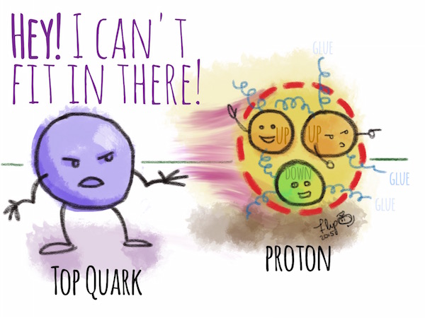
We know that protons are made up of two up quarks and a down quark. Each only weigh a few MeV—the rest of the proton mass comes from the strong force binding energy coming from gluon exchange. When we collider protons at high energies, these partons interact with each other to produce other particles. In fact, the LHC is essentially a gluon collider. Recently, however, physicists have been asking, “How much top quark is there in the proton?”
In fact, at first glance, this is a ridiculous question. The top quark is 175 times heavier than the proton! How does it make sense that there are top quarks “in” the proton?
The proton (1 GeV mass) doesn’t seem to have room for any top quark component (175 GeV mass).
Before we define what we mean by treating the top as a parton, we should define what we mean by proton! We can describe the proton constituents by a series of parton distribution functions (pdf): these tell us the probability of that you’ll interact with a particular piece of the proton. These pdfs are energy-dependent: at high energies, it turns out that you’re more likely to interact with a gluon than any of the “valence quarks.” At sufficiently high energies, these gluons can also produce pairs of heavier objects, like charm, bottom, and—at 100 TeV—even top quarks.
But there’s an even deeper sense in which these heavy quarks have a non-zero parton distribution function (i.e. “fraction of the proton”): it turns out that perturbation theory breaks down for certain kinematic regions when a gluon splits into quarks. That is to say, the small parameters we usually expand in become large.
Theoretically, a technique to keep the expansion parameter small leads to an interpretation of this “high-energy gluon splitting into heavy quarks inside the proton” process as the proton having some intrinsic heavy quark content. This is called perturbative QCD, the key equation known as DGLAP.
High energy gluon splittings can yield top quarks (lines with arrows). When one of these top quarks is collinear with the beam (pink, dashed), the calculation becomes non-perturbative. Maintaining the perturbation expansion parameter leads on to treat the top quark as a constituent of the proton. Solid blue lines are not-collinear and are well-behaved.
In the cartoon above: physically what’s happening is that a gluon in the proton splits into a top and anti-top. When one of these is collinear (i.e. goes down the collider beamline), the expansion parameter blows up and the calculation misbehaves. In order to maintain a well behaved perturbation theory, DGLAP tells us to pretend that instead of a top/anti-top pair coming from a gluon splitting, one can treat these as a top that lives inside the high-energy proton.
A gluon splitting that gives a non-perturvative top can be treated as a top inside the proton.
This is the sense in which the top quark can be considered as a parton. It doesn’t have to do with whether the top “fits” inside a proton and whether this makes sense given the mass—it boils down to a trick to preserve perturbativity.
One can recast this as the statement that the proton (or even fundamental particles like the electron) look different when you probe them at different energy scales. One can compare this story to this explanation for why the electron doesn’t have infinite electromagnetic energy.
The authors of 1411.2588 a study of the sensitivity a 100 TeV collider to processes that are produced from fusion of top quarks “in” each proton. With any luck, such a collider may even be on the horizon for future generations.
Figure 1: Monsieur Higgs boson hiding behind a background.
Last time I discussed the Higgs boson decay into photons, i.e. `shining light on the Higgs boson‘. This is a followup discussing more generally the problem of uncovering a Higgs boson which is hiding buried behind what can often be a large background (see Figure 1).
Perhaps the first question to ask is, what the heck is a background? Well, basically a background is anything that we `already know about’. In this case, this means the well understood Standard Model (SM) processes which do not involve a Higgs boson (which in this case is our `signal’), but can nevertheless mimic one of the possible decays of the Higgs. For most of these processes, we have very precise theoretical predictions in addition to previous experimental data from the LEP and Tevatron experiments (and others) which previously searched for the Higgs boson. So it is in reference to these non-Higgs SM processes when we use the term `background’.
As discussed in my previous post, the Higgs can decay to a variety of combinations of SM particles, which we call `channels’. Each of these channels has its own corresponding background which obscures the presence of a Higgs. For some channels the backgrounds are huge. For instance the background for a Higgs decaying to a pair of bottom quarks is so large (due to QCD) that, despite the fact this is the dominant decay channel (about 60% of Higgs’ decay to bottom quarks at 125 GeV), this channel has yet to be observed.
This is in contrast to the Higgs decay to four charged leptons (specifically electrons and muons) channel. This decay (mediated by a pair of virtual Z bosons) was one of the first discovery channels of the Higgs at the LHC despite the fact that roughly only one in every 10,000 Higgs bosons decays to four charge leptons. This is because this channel has a small background and is measured with very high precision. This high precision allows LHC experiments to scan over a range of energies in very small increments or `windows’. Since the background is very small, the probability of observing a background event in any given window is tiny. Thus, if an excess of events is seen in a particular window, this is an indication that there is a non background process occurring at that particular energy.
Figure 2: The energy spectrum of a Higgs decaying to four charged leptons (red) and its associated background (blue).
This is how the Higgs was discovered in the decay to four charged leptons at around 125 GeV. This can be seen in Figure 2 where in the window around the Higgs signal (shown in red) we see the background (shown in blue) is very small. Thus, once about a dozen events were observed at around 125 GeV, this was already enough evidence for experiments at the LHC to be able to claim discovery of the long sought after monsieur Higgs boson.
Over the past decade, a new trend has been emerging in physics, one that is motivated by several key questions: what do we know about the origin of our universe? What do we know about its composition? And how will the universe evolve from here? To delve into these questions naturally requires a thorough examination of the universe via the astrophysics lens. But studying the universe on a large scale alone does not provide a complete picture. In fact, it is just as important to see the universe on the smallest possible scales, necessitating the trendy and (fairly) new hybrid field of particle astrophysics. In this post, we will look specifically at the cosmic microwave background (CMB), classically known as a pillar of astrophysics, within the context of particle physics, providing a better understanding of the broader questions that encompass both fields.
Essentially, the CMB is just what we see when we look into the sky and we aren’t looking at anything else. Okay, fine. But if we’re not looking at something in particular, why do we see anything at all? The answer requires us to jump back a few billion years to the very early universe.
Figure 1: Particle interactions shown up to point of recombination, after which photon paths are unchanged.
Immediately after the Big Bang, it was impossible for particles to form atoms without immediately being broken apart by constant bombardment from stray photons. About 380,000 thousand years after the Big Bang, the Universe expanded and cooled to a temperature of about 3,000 K, allowing the first formation of stable hydrogen atoms. Since hydrogen is electrically neutral, the leftover photons could no longer interact, meaning that at that point their paths would remain unaltered indefinitely. These are the photons that we observe as CMB; Figure 1 shows this idea diagrammatically below. From our present observation point, we measure the CMB to have a temperature of about 2.76 K.
Since this radiation has been unimpeded since that specific point (known as the point of ‘recombination’), we can think of the CMB as a snapshot of the very early universe. It is interesting, then, to examine the regularity of the spectrum; the CMB is naturally not perfectly uniform, and the slight temperature variations can provide a lot of information about how the universe formed. In the early primordial soup universe, slight random density fluctuations exerted a greater gravitational pull on their surroundings, since they had slightly more mass. This process continues, and very large dense patches occur in an otherwise uniform space, heating up the photons in that area accordingly. The Planck satellite, launched in 2009, provides some beautiful images of the temperature anisotropies of the universe, as seen in Figure 2. Some of these variations can be quite severe, as in the recently released results about a supervoid aligned with an especially cold spot in the CMB (see Further Reading, item 4).
Figure 2: Planck satellite heat map images of the CMB.
Figure 3: Composition of the universe by percent.
So what does this all have to do with particles? We’ve talked about a lot of astrophysics so far, so let’s tie it all together. The big correlation here is dark matter. The CMB has given us strong evidence that our universe has a flat geometry, and from general relativity, this provides restrictions on the mass, energy, and density of the universe. In this way, we know that atomic matter can constitute only 5% of the universe, and analysis of the peaks in the CMB gives an estimate of 26% for the total dark matter presence. The rest of the universe is believed to be dark energy (see Figure 3).
Both dark matter and dark energy are huge questions in particle physics that could be the subject of a whole other post. But the CMB plays a big role in making our questions a bit more precise. The CMB is one of several pieces of strong evidence that require the existence of dark matter and dark energy to justify what we observe in the universe. Some potential dark matter candidates include weakly interacting massive particles (WIMPs), sterile neutrinos, or the lightest supersymmetric particle, all of which bring us back to particle physics for experimentation. Dark energy is not as well understood, and there are still a wide variety of disparate theories to explain its true identity. But it is clear that the future of particle physics will likely be closely tied to astrophysics, so as a particle physicist it’s wise to keep an eye out for new developments in both fields!
As we explained previously, IceCube is a gigantic ultra-high energy cosmic neutrino detector in Antarctica. These neutrinos have energies between 10-100 times higher than the protons colliding at the Large Hadron Collider, and their origin and nature are largely a mystery. One thing that IceCube can tell us about these neutrinos is their flavor composition; see e.g. this post for a crash course in neutrino flavor.
When neutrinos interact with ambient nuclei through a W boson (charged current interactions), the following types of events might be seen:
I refer you to this series of posts for a gentle introduction to the Feynman diagrams above. The key is that the high energy neutrino interacts with an nucleus, breaking it apart (the remnants are called X above) and ejecting a high energy charged lepton which can be used to identify the flavor of the neutrino.
Muons travel a long distance and leave behind a trail of Cerenkov radiation called a track.
Electrons don’t travel as far and deposit all of their energy into a shower. These are also sometimes called cascades because of the chain of particles produced in the ‘bang’.
Taus typically leave a more dramatic signal, a double bang, when the tau is formed and then subsequently decays into more hadrons (X’ above).
In fact, the tau events can be further classified depending on how this ‘double bang’ is resolved—and it seems like someone was playing a popular candy-themed mobile game when naming these:
Types of candy-themed tau events in IceCube from D. Cowan at the TeVPA 2 conference.
In this figure from the TeVPA 2 conference proceedings, we find some silly classifications of what tau events look like according to their energy:
Lollipop: The tau is produced outside the detector so that the first ‘bang’ isn’t seen. Instead, there’s a visible track that leads to the second (observable) bang. The track is the stick and the bang is the lollipop head.
Inverted lollipop: Similar to the lollipop, except now the first ‘bang’ is seen in the detector but the second ‘bang’ occurs outside the detector and is not observed.
Sugardaddy: The tau is produced outside the detector but decays into a muon inside the detector. This looks almost like a muon track except that the tau produces less Cerenkov light so that one can identify the point where the tau decays into a muon.
Double pulse: While this isn’t candy-themed, it’s still very interesting. This is a double bang where the two bangs can’t be distinguished spatially. However, since one bang occurs slightly after the other, one can distinguish them in the time: it’s a “double bang” in time rather than space.
Tautsie pop: This is a low energy version of the sugardaddy where the shower-to-track energy is used to discriminate against background.
While the names may be silly, counting these types of events in IceCube is one of the exciting frontiers of flavor physics. And while we might be forgiven for thinking that neutrino physics is all about measuring very `small’ things—let me share the following graphic from Francis Halzen’s recent talk at the AMS Days workshop at CERN, overlaying one of the shower events over Madison, Wisconsin to give a sense of scale:
Are cosmic neutrinos trying to tell us something, deep in the Antarctic ice?
Presenting:
“Glashow resonance as a window into cosmic neutrino sources,”
by Barger, Lu, Learned, Marfatia, Pakvasa, and Weiler Phys.Rev. D90 (2014) 121301 [1407.3255] Related work: Anchordoqui et al. [1404.0622], Learned and Weiler [1407.0739], Ibe and Kaneta [1407.2848]
Is there an neutrino energy cutoff preventing Glashow resonance events in IceCube?
The IceCube Neutrino Observatory is a gigantic neutrino detector located in the Antarctic. Like an iceberg, only a small fraction of the lab is above ground: 86 strings extend to a depth of 2.5 kilometers into the ice, with each string instrumented with 60 detectors.
2 PeV event from the IceCube 3 year analysis; nicknamed “Big Bird.” From 1405.5303.
These detectors search ultra high energy neutrinos by looking for Cerenkov radiation as they pass through the ice. This is really the optical version of a sonic boom. An example event is shown above, where the color and size of the spheres indicate the strength of the Cerenkov signal in each detector.
IceCube has released data for its first three years of running (1405.5303) and has found three events with very large energies: 1-2 peta-electron-volts: that’s ten thousand times the mass of the Higgs boson. In addition, there’s a spectrum of neutrinos in the 10-1000 TeV range.
Glashow resonance diagram.
These ultra high energy neutrinos are believed to originate from outside our galaxy through processes involving particle acceleration by black holes. One expects the flux of such neutrinos to go as a power law of the energy, where is a estimate from certain acceleration models. The existence of the three super high energy events at the PeV scale has led some people to think about a known deviation from the power law spectrum: the Glashow resonance. This is the sharp increase in the rate of neutrino interactions with matter coming from the resonant production of W bosons, as shown in the Feynman diagram to the left.
The Glashow resonance sticks out like a sore thumb in the spectrum. The position of the resonance is set by the energy required for an electron anti-neutrino to hit an electron at rest such that the center of mass energy is the W boson mass.
Sharp peak in the neutrino scattering rate from the Glashow resonance; image from Engel, Seckel, and Stanev in astro-ph/0101216.
If you work through the math on the back of an envelope, you’ll find that the resonance occurs for incident electron anti-neutrinos with an energy of 6.3 PeV; see figure to the leftt. This is “right around the corner” from the 1-2 PeV events already seen, and one might wonder whether it’s significant that we haven’t seen anything.
The authors of [1407.3255] have found that the absence of Glashow resonant neutrino events in IceCube is not yet a bona-fide “anomaly.” In fact, they point out that the future observation or non-observation of such neutrinos can give us valuable hints about the hard-to-study origin of these ultra high energy neutrinos. They present six simple particle physics scenarios for how high energy neutrinos can be formed from cosmic rays that were accelerated by astrophysical accelerators like black holes. Each of these processes predict a ratio of neutrino and anti-neutrinos flavors at Earth (this includes neutrino oscillation effects over long distances). Since the Glashow resonance only occurs for electronanti-neutrinos, the authors point out that the appearance or non-appearance of the Glashow resonance in future data can constrain what types of processes may have produced these high energy neutrinos.
In more speculative work, the authors of [1404.0622] suggest that the absence of Glashow resonance events may even suggest some kind of new physics that impose a “speed limit” on neutrinos propagating through space that prevents neutrinos from ever reaching 6.3 PeV (see top figure).
Further Reading:
1007.1247, Halzen and Klein, “IceCube: An Instrument for Neutrino Astronomy.” A review of the IceCube experiment.
hep-ph/9410384, Gaisser, Halzen, and Stanev, “Particle Physics with High Energy Neutrinos.” An older review of ultra high energy neutrinos.
Figure 1: Here we give a depiction of shining light on monsieur Higgs boson as well as demonstrate the extent of my french.
Hello Particle Nibblers,
This is my first Particlebites entry (and first ever attempt at a blog!) so you will have to bear with me =).
As I am sure you know by now, the Higgs boson has been discovered at the Large Hadron Collider (LHC). As you also may know, `discovering’ a Higgs boson is not so easy since a Higgs doesn’t just `sit there’ in a detector. Once it is produced at the LHC it very quickly decays (in about seconds) into other particles of the Standard Model. For us to `see’ it we must detect these particles into which decays. The decay I want to focus on here is the Higgs boson decay to a pair of photons, which are the spin-1 particles which make up light and mediate the electromagnetic force. By studying its decays to photons we are literally shining light on the Higgs boson (see Figure 1)!
The decay to photons is one of the Higgs’ most precisely measured decay channels. Thus, even though the Higgs only decays to photons about 0.2 % of the time, this was nevertheless one of the first channels the Higgs was discovered in at the LHC. Of course other processes (which we call backgrounds) in the Standard Model can mimic the decays of a Higgs boson, so to see the Higgs we have to look for `bumps’ over these backgrounds (see Figure 2). By carefully reconstructing this `bump’, the Higgs decays to photons also allows us to reconstruct the Higgs mass (about 125 GeV in particle physics units or about kg in `real world’ units).
Figure 2: Here we show the Higgs `bump’ in the invariant mass spectrum of the Higgs decay to a pair of photons.
Furthermore, using arguments based on angular momentum the Higgs decay to photons also allows us to determine that the Higgs boson must be a spin-0 particle which we call a scalar . So we see that just in this one decay channel a great deal of information about the Higgs boson can be inferred.
Now I know what you’re thinking…But photons only `talk to’ particles which carry electric charge and the Higgs is electrically neutral!! And even crazier, the Higgs only `talks to’ particles with mass and photons are massless!!! This is blasphemy!!! What sort of voodoo magic is occurring here which allows the Higgs boson to decay to photons?
The resolution of this puzzle lies in the subtle properties of quantum field theory. More specifically the Higgs can decay to photons via electrically charged `virtual particles‘. For present purposes its enough to say (with a little hand-waiving) that since the Higgs can talk to the massive electrically charged particles in the Standard Model, like the W boson or top quark, which in turn can `talk to’ photons, this allows the Higgs to indirectly interact with photons despite the fact that they are massless and the Higgs is neutral. In fact any charged and massive particles which exist will in principle contribute to the indirect interaction between the Higgs boson and photons. Crucially this includes even charged particles which may exist beyond the Standard Model and which have yet to be discovered due to their large mass. The sum total of these contributions from all possible charged and massive particles which contribute to the Higgs decay to photons is represented by the `blob’ in Figure 3.
Figure 3: Here we show how the Higgs decays to a pair of photons via `virtual charged particles’ (or more accurately disturbances in the quantum fields associated with these charge particles) represented by the grey`blob’.
It is exciting and interesting to think that new exotic charged particles could be hiding in the `blob’ which creates this interaction between the Higgs boson and photons. These particles might be associated with supersymmetry, extra dimensions, or a host of other exciting possibilities. So while it remains to be seen which, if any, of the beyond the Standard Model possibilities (please let there be something!) the LHC will uncover, it is fascinating to think about what can be learned by shining a little light on the Higgs boson!
Footnotes:
1. There is a possible exception to this if the Higgs is a spin-2 particle, but various theoretical arguments as well as other Higgs data make this scenario highly unlikely.
2. Note, virtual particle is unfortunately a misleading term since these are not really particles at all (really they are disturbances in their associated quantum fields), but I will avoid going down this rabbit hole for the time being and save it for a later post. See the previous `virtual particles’ link for a great and more in-depth discussion which takes you a little deeper into the rabbit hole.
Presenting: Section 3.2 of “Charged Lepton Flavor Violation: An Experimenter’s Guide” Authors: R. Bernstein, P. Cooper Reference: 1307.5787 (Phys. Rept. 532 (2013) 27)
Not all searches for new physics involve colliding protons at the the highest human-made energies. An alternate approach is to look for deviations in ultra-rare events at low energies. These deviations may be the quantum footprints of new, much heavier particles. In this bite, we’ll focus on the decay of a muon to an electron in the presence of a heavy atom.
Muons conversion into an electron in the presence of an atom, aluminum.
The muon is a heavy version of the electron.There are a few properties that make muons nice systems for precision measurements:
They’re easy to produce. When you smash protons into a dense target, like tungsten, you get lots of light hadrons—among them, the charged pions. These charged pions decay into muons, which one can then collect by bending their trajectories with magnetic fields. (Puzzle: why don’t pions decay into electrons? Answer below.)
They can replace electrons in atoms. If you point this beam of muons into a target, then some of the muons will replace electrons in the target’s atoms. This is very nice because these “muonic atoms” are described by non-relativistic quantum mechanics with the electron mass replaced with ~100 MeV. (Muonic hydrogen was previous mentioned in this bite on the proton radius problem.)
They decay, and the decay products always include an electron that can be detected. In vacuum it will decay into an electron and two neutrinos through the weak force, analogous to beta decay.
These decays are sensitive to virtual effects. You don’t need to directly create a new particle in order to see its effects. Potential new particles are constrained to be very heavy to explain their non-observation at the LHC. However, even these heavy particles can leave an imprint on muon decay through ‘virtual effects’ according (roughly) to the Heisenberg uncertainty principle: you can quantum mechanically violate energy conservation, but only for very short times.
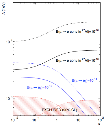
Reach of muon conversion experiments from 1303.4097. The y axis is the energy scale that can be probed and the x axis parameterizes different ways that lepton flavor violation can appear in a theory.
One should be surprised that muon conversion is even possible. The process cannot occur in vacuum because it cannot simultaneously conserve energy and momentum. (Puzzle: why is this true? Answer below.) However, this process is allowed in the presence of a heavy nucleus that can absorb the additional momentum, as shown in the comic at the top of this post.
Muon conversion experiments exploit this by forming muonic atoms in the 1s state and waiting for the muon to convert into an electron which can then be detected. The upside is that all electrons from conversion have a fixed energy because they all come from the same initial state: 1s muonic aluminum at rest in the lab frame. This is in contrast with more common muon decay modes which involve two neutrinos and an electron; because this is a multibody final state, there is a smooth distribution of electron energies. This feature allows physicists to distinguish between the conversion versus the more frequent muon decay in orbit or muon capture by the nucleus (similar to electron capture).
The Standard Model prediction for this rate is miniscule—it’s weighted by powers of the neutrino to the W boson mass ratio (Puzzle: how does one see this? Answer below.). In fact, the current experimental bound on muon conversion comes from the Sindrum II experiment looking at muonic gold which constrains the relative rate of muon conversion to muon capture by the gold nucleus to be less than . This, in turn, constrains models of new physics that predict some level of charged lepton flavor violation—that is, processes that change the flavor of a charged lepton, say going from muons to electrons.
The plot on the right shows the energy scales that are indirectly probed by upcoming muonic aluminum experiments: the Mu2e experiment at Fermilab and the COMET experiment at J-PARC. The blue lines show bounds from another rare muon decay: muons decaying into an electron and photon. The black solid lines show the reach for muon conversion in muonic aluminum. The dashed lines correspond to different experimental sensitivities (capture rates for conversion, branching ratios for decay with a photon). Note that the energy scales probed can reach 1-10 PeV—that’s 1000-10,000 TeV—much higher than the energy scales direclty probed by the LHC! In this way, flavor experiments and high energy experiments are complimentary searches for new physics.
These “next generation” muon conversion experiments are currently under construction and promise to push the intensity frontier in conjunction with the LHC’s energy frontier.
Solutions to exercises:
Why do pions decay into muons and not electrons? [Note: this requires some background in undergraduate-level particle physics.] One might expect that if a charged pion can decay into a muon and a neutrino, then it should also go into an electron and a neutrino. In fact, the latter should dominate since there’s much more phase space. However, the matrix element requires a virtual W boson exchange and thus depends on an [axial] vector current. The only vector available from the pion system is its 4-momentum. By momentum conservation this is $p_\pi = p_\mu + p_\nu$. The lepton momenta then contract with Dirac matrices on the leptonic current to give a dominant piece proportional to the lepton mass. Thus the amplitude for charged pion decay into a muon is much larger than the amplitude for decay into an electron.
Why can’t a muon decay into an electron in vacuum? The process cannot simultaneously conserve energy and momentum. This is simplest to see in the reference frame where the muon is at rest. Momentum conservation requires the electron to also be at rest. However, a particle has rest energy equal to its mass, but now there’s now way a muon at rest can pass on all of its energy to an electron at rest.
Why is muon conversion in the Standard Model suppressed by the ration of the neutrino to W masses? This can be seen by drawing the Feynman diagram (fig below from 1401.6077). Flavor violation in the Standard Model requires a W boson. Because the W is much heavier than the muon, this must be virtual and appear only as an internal leg. Further, W‘s couple charged leptons to neutrinos, so there must also be a virtual neutrino. The evaluation of this diagram into an amplitude gives factors of the neutrino mass in the numerator (required for the fermion chirality flip) and the W mass in the denominator. For some details, see this post.
Further Reading:
1205.2671: Fundamental Physics at the Intensity Frontier (section 3.2.2)
The Large Hadron Collider is the world’s largest proton collider, and in a mere five years of active data acquisition, it has already achieved fame for the discovery of the elusive Higgs Boson in 2012. Though the LHC is currently off to allow for a series of repairs and upgrades, it is scheduled to begin running again within the month, this time with a proton collision energy of 13 TeV. This is nearly double the previous run energy of 8 TeV, opening the door to a host of new particle productions and processes. Many physicists are keeping their fingers crossed that another big discovery is right around the corner. Here are a few specific things that will be important in Run II.
1. Luminosity scaling
Though this is a very general category, it is a huge component of the Run II excitement. This is simply due to the scaling of luminosity with collision energy, which gives a remarkable increase in discovery potential for the energy increase.
If you’re not familiar, luminosity is the number of events per unit time and cross sectional area. Integrated luminosity sums this instantaneous value over time, giving a metric in the units of 1/area.
In the particle physics world, luminosities are measured in inverse femtobarns, where 1 fb-1 = 1/(10-43 m2). Each of the two main detectors at CERN, ATLAS and CMS, collected 30 fb-1 by the end of 2012. The main point is that more luminosity means more events in which to search for new physics.
Figure 1 shows the ratios of LHC luminosities for 7 vs. 8 TeV, and again for 13 vs. 8 TeV. Since the plot is in log scale on the y axis, it’s easy to tell that 13 to 8 TeV is a very large ratio. In fact, 100 fb-1 at 8 TeV is the equivalent of 1 fb-1 at 13 TeV. So increasing the energy by a factor less than 2 increase the integrated luminosity by a factor of 100! This means that even in the first few months of running at 13 TeV, there will be a huge amount of data available for analysis, leading to the likely release of many analyses shortly after the beginning of data acquisition.
Figure 1: Parton luminosity ratios, from J. Stirling at Imperial College London (see references.)
2. Supersymmetry
Supersymmetry theory proposes the existence of a superpartner for every particle in the Standard Model, effectively doubling the number of fundamental particles in the universe. This helps to answer many questions in particle physics, namely the question of where the particle masses came from, known as the ‘hierarchy’ problem (see the further reading list for some good explanations.)
Current mass limits on many supersymmetric particles are getting pretty high, concerning some physicists about the feasibility of finding evidence for SUSY. Many of these particles have already been excluded for masses below the order of a TeV, making it very difficult to create them with the LHC as is. While there is talk of another LHC upgrade to achieve energies even higher than 14 TeV, for now the SUSY searches will have to make use of the energy that is available.
Figure 2: Cross sections for the case of equal degenerate squark and gluino masses as a function of mass at √s = 13 TeV, from 1407.5066. q stands for quark, g stands for gluino, and t stands for stop.
Figure 2 shows the cross sections for various supersymmetric particle pair production, including squark (the supersymmetric top quark) and gluino (the supersymmetric gluon). Given the luminosity scaling described previously, these cross sections tell us that with only 1 fb-1, physicists will be able to surpass the existing sensitivity for these supersymmetric processes. As a result, there will be a rush of searches being performed in a very short time after the run begins.
3. Dark Matter
Dark matter is one of the greatest mysteries in particle physics to date (see past particlebites posts for more information). It is also one of the most difficult mysteries to solve, since dark matter candidate particles are by definition very weakly interacting. In the LHC, potential dark matter creation is detected as missing transverse energy (MET) in the detector, since the particles do not leave tracks or deposit energy.
One of the best ways to ‘see’ dark matter at the LHC is in signatures with mono-jet or photon signatures; these are jets/photons that do not occur in pairs, but rather occur singly as a result of radiation. Typically these signatures have very high transverse momentum (pT) jets, giving a good primary vertex, and large amounts of MET, making them easier to observe. Figure 3 shows a Feynman diagram of such a decay, with the MET recoiling off a jet or a photon.
Figure 3: Feynman diagram of mono-X searches for dark matter, from “Hunting for the Invisible.”
Though the topics in this post will certainly be popular in the next few years at the LHC, they do not even begin to span the huge volume of physics analyses that we can expect to see emerging from Run II data. The next year alone has the potential to be a groundbreaking one, so stay tuned!
Last Thursday, Nobel Laureate Sam Tingpresented the latest results (CERN press release) from the Alpha Magnetic Spectrometer (AMS-02) experiment, a particle detector attached to the International Space Station—think “ATLAS/CMS in space.” Instead of beams of protons, the AMS detector examines cosmic rays in search of signatures of new physics such as the products of dark matter annihilation in our galaxy.
In fact, this is just the latest chapter in an ongoing mystery involving the energy spectrum of cosmic positrons. Recall that positrons are the antimatter versions of electrons with identical properties except having opposite charge. They’re produced from known astrophysical processes when high-energy cosmic rays (mostly protons) crash into interstellar gas—in this case they’re known as `secondaries’ because they’re a product of the `primary’ cosmic rays.
The dynamics of charged particles in the galaxy are difficult to simulate due to the presence of intense and complicated magnetic fields. However, the diffusion models generically predict that the positron fraction—the number of positrons divided by the total number of positrons and electrons—decreases with energy. (This ratio of fluxes is a nice quantity because some astrophysical uncertainties cancel.)
This prediction, however, is in stark contrast with the observed positron fraction from recent satellite experiments:
Observed positron fraction from recent experiments compared to expected astrophysical background (gray) from APS viewpoint article based on the 2013 AMS-02 results (data) and the analysis in 1002.1910 (background).
The rising fraction had been hinted in balloon-based experiments for several decades, but the satellite experiments have been able to demonstrate this behavior conclusively because they can access higher energies. In their first set of results last year (shown above), AMS gave the most precise measurements of the positron fraction as far as 350 GeV. Yesterday’s announcement extended these results to 500 GeV and added the following observations:
First they claim that they have measured the maximum of the positron fraction to be 275 GeV. This is close to the edge of the data they’re releasing, but the plot of the positron fraction slope is slightly more convincing:
Lower: the latest positron fraction data from AMS-02 against a phenomenological model. Upper: slope of the lower curve. From Phys. Rev. Lett. 113, 121101. [Non-paywall summary.]The observation of a maximum in what was otherwise a fairly featureless rising curve is key for interpretations of the excess, as we discuss below. A second observation is a bit more curious: while neither the electron nor the positron spectra follow a simple power law, , the total electron or positron flux does follow such a power law over a range of energies.
Total electron/positron flux weighted by the cubed energy and the fit to a simple power law. From the AMS press summary.
This is a little harder to interpret since the flux form electrons also, in principle, includes different sources of background. Note that this plot reaches higher energies than the positron fraction—part of the reason for this is that it is more difficult to distinguish between electrons and positrons at high energies. This is because the identification depends on how the particle bends in the AMS magnetic field and higher energy particles bend less. This, incidentally, is also why the FERMI data has much larger error bars in the first plot above—FERMI doesn’t have its own magnetic field and must rely on that of the Earth for charge discrimination.
So what should one make of the latest results?
The most optimistic hope is that this is a signal of dark matter, and at this point this is more of a ‘wish’ than a deduction. Independently of AMS, we know is that dark matter exists in a halo that surrounds our galaxy. The simplest dark matter models also assume that when two dark matter particles find each other in this halo, they can annihilate into Standard Model particle–anti-particle pairs, such as electrons and positrons—the latter potentially yielding the rising positron fraction signal seen by AMS.
From a particle physics perspective, this would be the most exciting possibility. The ‘smoking gun’ signature of such a scenario would be a steep drop in the positron fraction at the mass of the dark matter particle. This is because the annihilation occurs at low velocities so that the energy of the annihilation products is set by the dark matter mass. This is why the observation of a maximum in the positron fraction is interesting: the dark matter interpretation of this excess hinges on how steeply the fraction drops off.
There are, however, reasons to be skeptical.
One attractive feature of dark matter annihilations is thermal freeze out: the observation that the annihilation rate determines how much dark matter exists today after being in thermal equilibrium in the early universe. The AMS excess is suggestive of heavy (~TeV scale) dark matter with an annihilation rate three orders of magnitude larger than the rate required for thermal freeze out.
A study of the types of spectra one expects from dark matter annihilation shows fits that are somewhat in conflict with the combined observations of the positron fraction, total electron/positron flux, and the anti-proton flux (see 0809.2409). The anti-proton flux, in particular, does not have any known excess that would otherwise be predicted by dark matter annihilation into quarks.
There are ways around these issues, such as invoking mechanisms to enhance the present day annihilation rate, perhaps with the annihilation only creating leptons and not quarks. However, these are additional bells and whistles that model-builders must impose on the dark matter sector. It is also important to consider alternate explanations of the Pamela/FERMI/AMS positron fraction excess due to astrophysical phenomena. There are at least two very plausible candidates:
Pulsars are neutron stars that are known to emit “primary” electron/positron pairs. A nearby pulsar may be responsible for the observed rising positron fraction. See 1304.1791 for a recent discussion.
Alternately, supernova remnants may also generate a “secondary” spectrum of positrons from acceleration along shock waves (0909.4060, 0903.2794, 1402.0855).
Both of these scenarios are plausible and should temper the optimism that the rising positron fraction represents a measurement of dark matter. One useful handle to disfavor the astrophysical interpretations is to note that they would be anisotropic (not constant over all directions) whereas the dark matter signal would be isotropic. See 1405.4884 for a recent discussion. At the moment, the AMS measurements do not measure any anisotropy but are not yet sensitive enough to rule out astrophysical interpretations.
Finally, let us also point out an alternate approach to understand the positron fraction. The reason why it’s so difficult to study cosmic rays is that the complex magnetic fields in the galaxy are intractable to measure and, hence, make the trajectory of charged particles hopeless to trace backwards to their sources. Instead, the authors of 0907.1686 and 1305.1324 take an alternate approach: while we can’t determine the cosmic ray origins, we can look at the behavior of heavier cosmic ray particles and compare them to the positrons. This is because, as mentioned above, the bending of a charged particle in a magnetic field is determined by its mass and charge—quantities that are known for the various cosmic ray particles. Based on this, the authors are able to predict an upper bound for the positron fraction when one assumes that the positrons are secondaries (e.g in the case of supernovae remnant acceleration):
We see that the AMS-02 spectrum is just under the authors’ upper bound, and that the reported downturn is consistent with (even predicted from) the upper-bound. The authors’ analysis then suggests a non-dark matter explanation for the positron excess. See this post from Resonaances for a discussion of this point and an updated version of the above plot from the authors.
With that in mind, there are at least three things to look forward to in the future from AMS:
A corresponding upturn in the anti-proton flux is predicted in many types of dark matter annihilation models for the rising positron fraction. Thus far AMS-02 has not released anti-proton data due to the lower numbers of anti-protons.
Further sensitivity to the (an)isotropy of the excess is a critical test of the dark matter interpretation.
The shape of the drop-off with energy is also critical: a gradual drop-off is unlikely to come from dark matter whereas a steep drop off is considered to be a smoking gun for dark matter.
Only time will tell; though Ting suggested that new results would be presented at the upcoming AMS meeting at CERN in 2 months.
Further reading:
The recent Sackler Symposium on the Nature of Dark matter included three talks on various aspects of the Pamela/FERMI/AMS-02 rising positron fraction. You can view the videos here: Linden (pulsars), Galli (dark matter), Blum (upper bound on secondaries).
The APS Physics journal has a nice synopsis article on this year’s AMS-02 results; see also their more extensive viewpoint article from last year’s results.
For a more hands-on introduction to indirect detection of dark matter, see Stefano Profumo’s 2012 TASI lectures with particular attention to lecture 3.


 where
where  is a estimate from
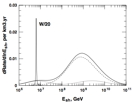

 seconds) into other particles of the
  kg in `real world’ units).
 . So we see that just in this one decay channel a great deal of information about the Higgs boson can be inferred.
 . For present purposes its enough to say (with a little hand-waiving) that since the Higgs can talk to the massive electrically charged particles in the Standard Model, like the

 cannot occur in vacuum because it cannot simultaneously conserve energy and momentum. (Puzzle: why is this true?
  in orbit or muon capture by the nucleus (similar to
  . This, in turn, constrains models of new physics that predict some level of charged lepton flavor violation—that is, processes that change the flavor of a charged lepton, say going from muons to electrons.
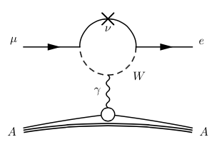


 , the total electron or positron flux does follow such a power law over a range of energies.
